Create a Price Spike Forecast Model
This tutorial will walk you through how to predict price spikes in ERCOT
Tutorial Overview
This tutorial will walk you through creating a model for forecasting spikes in ERCOT's Real Time Market (RTM) System Lambda price. We'll focus on the the day ahead horizon, where we'll predict real time price spikes before the Day Ahead Market (DAM) closes.
Along the way, we'll put several key platform features to use, including:
- Third-Party Data through Source Connectors
- XGBoost through Model Connectors
- Time Series Layering
- Backtesting
Note: You'll need access to Yes Energy's Full data share to access all of the datatypes in this tutorial. If you're interested in getting access, feel free to reach out to [email protected].
Create your NoTS
For this tutorial, you will leverage the client library to create your NoTS. The NoTS that you'll create will use an XGBoost model with a variety of features to forecast spikes in ERCOT's RTM System Lambda price.
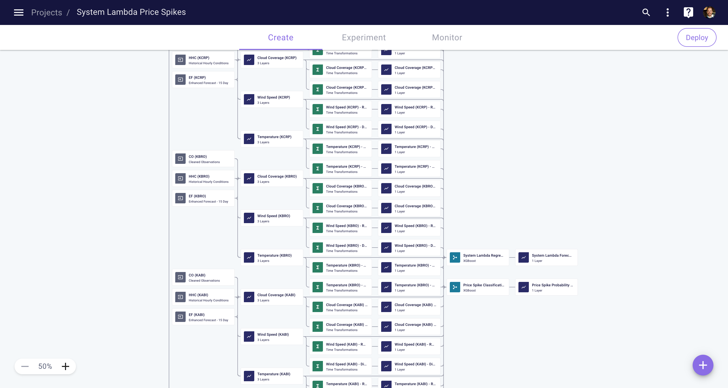
The Network of Time Series (NoTS) that you'll create in this tutorial
Features
A forecasting system is only as good as the data you give it. At Myst, we typically use the following data types to model market prices:
- Market Data
- Price data — Recent prices are very strong predictors of tomorrow's price. In particular, we can use the RTM price from yesterday and the DAM price for the current day to predict the RT price for tomorrow.
- Load data — These can be forecasts or recent past actuals, for the whole system and at the zonal level.
- Renewable generation data — Similarly to load, these can be forecasts or recent past actuals, for the whole system and at the zonal level. In ERCOT, the renewable generation type of interest is primarily wind generation, but we'll include solar here as well.
- Generation capacity forecasts — We'll use ERCOT's forecasts for how much generation capacity will be available, as well as previous day's actual capacity in the DA market and real time operations.
- Weather Data
- This includes temperature, wind, and cloud coverage, which provide supplemental information about load, wind, and solar generation, respectively.
- Time-Based Data
- Prices vary with the hour of day and season of year, so we use features indicating those timings in our models.
Below, we'll go through how to incorporate each of these feature types step by step.
Imports and Helper Functions
First thing's first, let's get our imports in order and define some useful constants.
from typing import List, Optional
from typing import Tuple

import myst
import pandas
from myst.connectors.model_connectors import xgboost
from myst.connectors.operation_connectors import numerical_expression
from myst.connectors.operation_connectors import time_transformations
from myst.connectors.source_connectors import time_trends
from myst.connectors.source_connectors import yes_energy
from myst.models.enums import OrgSharingRole
from myst.recipes.time_series_recipes import the_weather_company
from myst.resources.node import Node

SAMPLE_PERIOD = myst.TimeDelta("PT1H")
TIME_ZONE = "US/Central"
Next, we'll define some utils and time series operations that will apply to the whole tutorial.
def get_time_series_by_title(nodes: List[Node], title: str) -> myst.TimeSeries:
    """Gets a time series with the specified title from the list of nodes.

    Args:
        nodes: list of nodes
        title: title to filter for

    Returns:
        the time series with the specified title
    """
    for node in nodes:
        if isinstance(node, myst.TimeSeries) and node.title == title:
            return node

    raise ValueError("No time series with requested title found.")


def create_lag_feature(
    project: myst.Project, time_series: myst.TimeSeries, lag_period: myst.TimeDelta
) -> myst.TimeSeries:
    """Creates a new time series that lags the input by the lag period.

    Args:
        project: the project to add the operation and time series nodes to.
        time_series: the time series to apply the operation to.
        lag_period: the period to lag the time series by.

    Returns:
        the resulting time series
    """
    title = f"{time_series.title} - Lag {lag_period.to_iso_string()}"
    operation = project.create_operation(
        title=title,
        connector=time_transformations.TimeTransformations(
            shift_parameters=time_transformations.ShiftParameters(shift_period=lag_period)
        ),
    )
    operation.create_input(time_series=time_series, group_name=time_transformations.GroupName.OPERANDS)

    return operation.create_time_series(title=title, sample_period=SAMPLE_PERIOD)


def create_first_order_difference_feature(
    project: myst.Project, time_series: myst.TimeSeries, differencing_period: myst.TimeDelta
) -> myst.TimeSeries:
    """Creates a new time series by applying a first order difference on the input over the differencing period.

    Args:
        project: the project to add the operation and time series nodes to.
        time_series: the time series to apply the operation to.
        differencing_period: the period to difference the time series on.

    Returns:
        the resulting time series
    """
    title = f"{time_series.title} - Diff {differencing_period.to_iso_string()}"
    connector = time_transformations.TimeTransformations(
        differencing_parameters=time_transformations.DifferencingParameters(
            differencing_period=differencing_period, differencing_order=1
        )
    )
    operation = project.create_operation(title=title, connector=connector)
    operation.create_input(time_series=time_series, group_name=time_transformations.GroupName.OPERANDS)

    return operation.create_time_series(title=title, sample_period=SAMPLE_PERIOD)


def create_rolling_mean_feature(
    project: myst.Project, time_series: myst.TimeSeries, window_period: myst.TimeDelta
) -> myst.TimeSeries:
    """Creates a new time series by applying a rolling mean on the input over the window period.

    Args:
        project: the project to add the operation and time series nodes to.
        time_series: the time series to apply the operation to.
        window_period: the window period to apply the rolling mean over.

    Returns:
        the resulting time series
    """
    title = f"{time_series.title} - Rolling Mean {window_period.to_iso_string()}"
    connector = time_transformations.TimeTransformations(
        rolling_window_parameters=time_transformations.RollingWindowParameters(
            window_period=window_period,
            min_periods=1,
            centered=False,
            aggregation_function=time_transformations.AggregationFunction.MEAN,
        )
    )
    operation = project.create_operation(title=title, connector=connector)
    operation.create_input(time_series=time_series, group_name=time_transformations.GroupName.OPERANDS)

    return operation.create_time_series(title=title, sample_period=SAMPLE_PERIOD)
Market Data
Yes Energy is our primary third-pary data provider for market data. They collect and normalize ISO-provided data including prices and forecasted and actual operations data, among other things. We'll make heavy use of our Yes Energy source connector in the following sections.
# Yes Energy object IDs for locations of interest in ERCOT.
ERCOT_ISO_ZONE = 10000756298
ERCOT_LOAD_ZONE = 10000712973

FAR_WEST_WEATHER_ZONE = 10002211347
NORTH_CENTRAL_WEATHER_ZONE = 10002211349
NORTH_WEATHER_ZONE = 10002211348
SOUTHERN_WEATHER_ZONE = 10002211351

COASTAL_GENERATION_REGION = 10004189446
ERCOT_GENERATION_REGION = 10004189442
PANHANDLE_GENERATION_REGION = 10004189445
SOUTHERN_GENERATION_REGION = 10004189447
WEST_GENERATION_REGION = 10004189450

# The offset to use for all Yes Energy forecast types. The format is DD:HH:MM indicating that the forecasts to be queried should
# be available DD days before the forecasted time at or before HH:MM.
# This offset will query forecasts available as-of the prior day to the datetime being forecasted, at or before 09:00
# local time.
FORECAST_VINTAGE_OFFSET = "01:09:00"
Price Data
Here we're requesting the real-time system lambda and the system lambda of the DAM from Yes Energy. The system lambda time series will be our target to predict, and we create some lagged time series of the RT and DA system lambdas to be used as features.
def create_system_lambda_and_create_features(project: myst.Project) -> Tuple[myst.TimeSeries, List[myst.TimeSeries]]:
    """Queries the system lambda price and creates associated lag features.

    Args:
        project: the project to add the source and time series to.

    Returns:
        tuple of (system lambda, lagged system lambda features).
    """
    system_lambda_items = [
        yes_energy.YesEnergyItem("SYSTEM_LAMBDA", ERCOT_ISO_ZONE),
        yes_energy.YesEnergyItem("SYSTEM_LAMBDA_DA", ERCOT_ISO_ZONE),
    ]
    source = project.create_source(title="System Lambdas", connector=yes_energy.YesEnergy(items=system_lambda_items))
    system_lambda = source.create_time_series(
        title="System Lambda", label_indexer=f"SYSTEM_LAMBDA_{ERCOT_ISO_ZONE}", sample_period=SAMPLE_PERIOD
    )
    system_lambda_da = source.create_time_series(
        title="System Lambda DA", label_indexer=f"SYSTEM_LAMBDA_DA_{ERCOT_ISO_ZONE}", sample_period=SAMPLE_PERIOD
    )

    # If today, we're predicting the price tomorrow, we can use yesterday's RT price and today and yesterday's DA price.
    # The lag periods are with respective to the forecasted time (tomorrow), so a 48-hour lag gives the value of the
    # price 2 days before the time that we're forecasting.
    features = [
        create_lag_feature(project=project, time_series=system_lambda, lag_period=myst.TimeDelta("PT48H")),
        create_lag_feature(project=project, time_series=system_lambda_da, lag_period=myst.TimeDelta("PT24H")),
        create_lag_feature(project=project, time_series=system_lambda_da, lag_period=myst.TimeDelta("PT48H")),
    ]

    return system_lambda, features
Load Data
Next, we'll request load forecasts from Yes Energy for ERCOT as a whole, as well as the Far West, North, North Central, and Southern weather zones.
Whenever we deal with forecast features, we have to be cognizant of the so called "as of time" of the forecast. That is, we need to be sure that the forecast features we use for prediction will be available as of the time that we generate our price forecasts. Additionally, when we evaluate these forecasts in a backtest, we need to make sure that the feature data used in the backtest would have been available at the time we would have generated our forecasts.
We can use layering to accomplish both of these goals. We'll create a single time series with two layers:
- The top, highest precedence layer will query the most recently available (i.e. freshest) forecasts. We'll configure the timing of this layer to only apply to future timestamps. This way, whenever we make forecasts into the future, we'll be using the freshest forecasts available.
- The bottom, lower precedence layer will query the forecasts that were available as of the prior day, at or before 09:00, with respect to the timestamp that we're forecasting. The layer is configured to only apply to historical timestamps, so it'll only be used in the training data and in backtesting. For consistency, we'll also configure our backtests to simulate generating forecasts daily at 09:00 for the next day's real-time prices.
Finally, we also add some feature engineering in the form of differenced load. Specifically, we're creating a feature that represents the difference between tomorrow's load forecast and today's load forecast. At Myst, we've found feature difference like this to be helpful, but you should feel free to explore your own feature engineering approaches!
def create_load_features(project: myst.Project) -> List[myst.TimeSeries]:
    """Creates the load forecast features.

    Args:
        project: the project to add the source, operation, and time series to.

    Returns:
        list of feature time series.
    """
    latest_forecast_items = [
        yes_energy.YesEnergyItem("LOAD_FORECAST", ERCOT_LOAD_ZONE),
        yes_energy.YesEnergyItem("LOAD_FORECAST", FAR_WEST_WEATHER_ZONE),
        yes_energy.YesEnergyItem("LOAD_FORECAST", NORTH_CENTRAL_WEATHER_ZONE),
        yes_energy.YesEnergyItem("LOAD_FORECAST", NORTH_WEATHER_ZONE),
        yes_energy.YesEnergyItem("LOAD_FORECAST", SOUTHERN_WEATHER_ZONE),
    ]
    latest_forecast_source = project.create_source(
        title="Latest Load Forecasts", connector=yes_energy.YesEnergy(items=latest_forecast_items)
    )

    # Query the load forecasts that were available as of the forecast vintage offset.
    before_dam_close_forecast_items = [
        yes_energy.YesEnergyItem(item.datatype, item.object_id, forecast_vintage_offset=FORECAST_VINTAGE_OFFSET)
        for item in latest_forecast_items
    ]
    before_dam_close_forecast_source = project.create_source(
        title="Pre-DAM Close Load Forecasts", connector=yes_energy.YesEnergy(items=before_dam_close_forecast_items)
    )

    # For each zonal load forecast, we'll create a layered time series. The top layer will be the latest available
    # forecasts, while the bottom layer will be the forecasts available as of the previous day at 09:00 local time.
    features = []
    for item in latest_forecast_items:
        title = f"{item.datatype}_{item.object_id}"
        time_series = project.create_time_series(title=title, sample_period=SAMPLE_PERIOD)

        # The start timing ensures that this layer's data will only be used when making forecasts into the future.
        time_series.create_layer(
            node=latest_forecast_source,
            order=0,
            label_indexer=title,
            start_timing=myst.TimeDelta("PT1H"),
        )

        # The end timing ensures that this layer's data will only be used when backcasting, e.g. during a backtest.
        time_series.create_layer(
            node=before_dam_close_forecast_source,
            order=1,
            label_indexer=f"{title}@{FORECAST_VINTAGE_OFFSET}",
            end_timing=myst.TimeDelta("PT0H"),
        )

        difference_time_series = create_first_order_difference_feature(
            project=project, time_series=time_series, differencing_period=myst.TimeDelta("PT24H")
        )

        features.extend([time_series, difference_time_series])

    return features
Renewable Generation Data
Very much like load forecasts, we'll query wind and solar generation forecasts from Yes Energy. The following function uses the same layering logic as above to ensure that the forecast data in our graphs is always the most recently available forecast as of the actual or simulated prediction time.
def create_renewable_generation_features(project: myst.Project) -> List[myst.TimeSeries]:
    """Creates the renewable generation forecast features.

    Args:
        project: the project to add the source, operation, and time series to.

    Returns:
        list of feature time series.
    """
    # Query the latest available renewable generation forecasts.
    latest_forecast_items = [
        yes_energy.YesEnergyItem("WIND_COPHSL", ERCOT_GENERATION_REGION),
        yes_energy.YesEnergyItem("WIND_COPHSL", COASTAL_GENERATION_REGION),
        yes_energy.YesEnergyItem("WIND_COPHSL", PANHANDLE_GENERATION_REGION),
        yes_energy.YesEnergyItem("WIND_COPHSL", SOUTHERN_GENERATION_REGION),
        yes_energy.YesEnergyItem("WIND_COPHSL", WEST_GENERATION_REGION),
        yes_energy.YesEnergyItem("SOLAR_COPHSL", ERCOT_LOAD_ZONE),
    ]
    latest_forecast_source = project.create_source(
        title="Latest Renewable Generation Forecasts",
        connector=yes_energy.YesEnergy(items=latest_forecast_items),
    )

    before_dam_close_forecast_items = [
        yes_energy.YesEnergyItem(item.datatype, item.object_id, forecast_vintage_offset=FORECAST_VINTAGE_OFFSET)
        for item in latest_forecast_items
    ]
    before_dam_close_forecast_source = project.create_source(
        title="Pre-DAM Close Renewable Generation Forecasts",
        connector=yes_energy.YesEnergy(items=before_dam_close_forecast_items),
    )

    features = []
    for item in latest_forecast_items:
        title = f"{item.datatype}_{item.object_id}"
        time_series = project.create_time_series(title=title, sample_period=SAMPLE_PERIOD)
        time_series.create_layer(
            node=latest_forecast_source,
            order=0,
            label_indexer=title,
            start_timing=myst.TimeDelta("PT1H"),
        )
        time_series.create_layer(
            node=before_dam_close_forecast_source,
            order=1,
            label_indexer=f"{title}@{FORECAST_VINTAGE_OFFSET}",
            end_timing=myst.TimeDelta("PT0H"),
        )

        features.append(time_series)

        if "WIND" in title:
            features.append(
                create_lag_feature(project=project, time_series=time_series, lag_period=myst.TimeDelta("PT1H"))
            )

    return features
Generation Capacity Data
In this section, we'll query three datatypes that fall under the "generation capacity" umbrella:
HSL_DA: The total high sustainable load from all generating resources in the DAM runRT_ON_CAP: The real-time online capacity of the ERCOT systemGEN_RESOURCE: A forecast of the generation capacity in ERCOT
Note that you will need access to Yes Energy's Full Date Share to query these datatypes. If you do not have access, you can skip this bit of code.
When you query the RT_ON_CAP data, you'll see it's not actually the total system capacity (it's not the right order of magnitude). It's actually the system reserves, the amount of capacity available in addition to the load that is currently being served. We've found that this delta between total capacity and load is especially helpful for predicting price spikes. The following function creates features representing the delta between capacity and load for the DAM capacity (HSL_DA) and the forecasted generation capacity (GEN_RESOURCE).
For the forecasted generation capacity data, we'll use the same layering logic as above to ensure we only use forecast data that is available as of the actual or simulated prediction time.
def create_capacity_features(project: myst.Project, ercot_load_forecast: myst.TimeSeries) -> List[myst.TimeSeries]:
    """Creates the generation capacity features.

    Args:
        project: the project to add the source, operation, and time series nodes to.
        ercot_load_forecast: the time series containing load forecasts for all of ERCOT.

    Returns:
        list of feature time series.
    """
    capacity_items = [
        yes_energy.YesEnergyItem("HSL_DA", ERCOT_LOAD_ZONE),
        yes_energy.YesEnergyItem("RT_ON_CAP", ERCOT_ISO_ZONE),
        yes_energy.YesEnergyItem("GEN_RESOURCE", ERCOT_ISO_ZONE),
        yes_energy.YesEnergyItem("GEN_RESOURCE", ERCOT_ISO_ZONE, forecast_vintage_offset=FORECAST_VINTAGE_OFFSET),
    ]
    source = project.create_source(title="Generation Capacity", connector=yes_energy.YesEnergy(items=capacity_items))

    capacity_time_series = []

    # Handle the non-forecasts first.
    for item in capacity_items[:2]:
        title = f"{item.datatype}_{item.object_id}"
        capacity_time_series.append(
            source.create_time_series(title=title, label_indexer=title, sample_period=SAMPLE_PERIOD)
        )

    # Layer the forecast data.
    gen_resource_title = f"GEN_RESOURCE_{ERCOT_ISO_ZONE}"
    time_series = project.create_time_series(title=gen_resource_title, sample_period=SAMPLE_PERIOD)
    time_series.create_layer(
        node=source,
        order=0,
        label_indexer=gen_resource_title,
        start_timing=myst.TimeDelta("PT1H")
    )
    time_series.create_layer(
        node=source,
        order=1,
        label_indexer=f"{gen_resource_title}@{FORECAST_VINTAGE_OFFSET}",
        end_timing=myst.TimeDelta("PT0H"),
    )
    capacity_time_series.append(time_series)

    def _capacity_load_delta_feature(capacity, load):
        """Creates feature representing the delta between total generation capacity and load."""
        operation = project.create_operation(
            title=f"{capacity.title} - {load.title}",
            connector=numerical_expression.NumericalExpression(
                variable_names=["capacity", "load"], math_expression="capacity - load"
            ),
        )
        operation.create_input(time_series=capacity, group_name="capacity")
        operation.create_input(time_series=load, group_name="load")

        return operation.create_time_series(title=f"{capacity.title}_{load.title} Delta", sample_period=SAMPLE_PERIOD)

    hsl_load_delta = _capacity_load_delta_feature(capacity_time_series[0], ercot_load_forecast)
    gen_resource_load_delta = _capacity_load_delta_feature(capacity_time_series[2], ercot_load_forecast)

    features = [
        # Lag the HSL and RT_ON_CAP series since these are actual values that won't be available for the future times.
        create_lag_feature(project=project, time_series=hsl_load_delta, lag_period=myst.TimeDelta("PT24H")),
        create_lag_feature(project=project, time_series=capacity_time_series[1], lag_period=myst.TimeDelta("PT48H")),
        gen_resource_load_delta,
        create_first_order_difference_feature(
            project=project, time_series=gen_resource_load_delta, differencing_period=myst.TimeDelta("PT24H")
        ),
    ]

    return features
Weather Data
For weather data, we'll user our Atmospheric G2 (AG2), formerly The Weather Company, recipe to query the temperature, wind speed, and cloud coverage of several METAR stations across Texas. We'll also apply some standard time series feature engineering transformations, like 24-hour differencing and 24-hour rolling means.
Unfortunately, AG2 doesn't store historical forecasts associated with as-of times. That means that we can't query weather forecasts available as of prediction time and apply the same layering approach as we used above. Instead training and backtesting will use actual weather data. The AG2 recipe handles the nuances of creating separate layers for historical actuals and future forecasts, but it's still an important detail to keep in mind when interpreting backtesting results.
def create_weather_features(project: myst.Project) -> List[myst.TimeSeries]:
    """Creates the weather features.

    Args:
        project: the project to add the source, operation, and time series to.

    Return:
        list of feature time series.
    """
    weather_metars = [
        the_weather_company.MetarStation.KABI,  # Austin
        the_weather_company.MetarStation.KBRO,  # Brownsville
        the_weather_company.MetarStation.KCRP,  # Corpus Christi
        the_weather_company.MetarStation.KDFW,  # Dallas
        the_weather_company.MetarStation.KIAH,  # Houston
    ]
    weather_fields = [
        the_weather_company.Field.TEMPERATURE,
        the_weather_company.Field.WIND_SPEED,
        the_weather_company.Field.CLOUD_COVERAGE,
    ]
    features = []
    for metar in weather_metars:
        for field in weather_fields:
            ts = project.create_time_series_from_recipe(
                recipe=the_weather_company.TheWeatherCompany(metar_station=metar, field=field)
            )
            differenced = create_first_order_difference_feature(
                project=project, time_series=ts, differencing_period=myst.TimeDelta("PT24H")
            )
            rolling_mean = create_rolling_mean_feature(
                project=project, time_series=ts, window_period=myst.TimeDelta("PT24H")
            )
            features.extend([ts, differenced, rolling_mean])

    return features
Time-Based Data
For our final feature category, we'll create time series for the epoch, hour of day, day of week, and day of year. The last 3 features can help correlate price spikes to periodic changes in load throughout the day, week, and year. For example, price spikes often happen in the late afternoon and in the hot summer months when load is at its highest.
The epoch feature is an interesting one. It is a timeseries counting up the number of seconds since the epoch (January 1, 1970). This feature captures where we are in time. Specifically for tree models, it gives us a feature to split on when there are major differences in the behavior of a time series signal before and after certain dates.
def create_time_trends_features(project: myst.Project) -> List[myst.TimeSeries]:
    """Create the time trends features.

    Args:
        project: the project to add the source and time series to.

    Returns:
        list of feature time series.
    """
    time_trends_fields = [
        time_trends.Field.EPOCH,
        time_trends.Field.HOUR_OF_DAY,
        time_trends.Field.DAY_OF_WEEK,
        time_trends.Field.DAY_OF_YEAR,
    ]
    source = project.create_source(
        title="Time Trends",
        connector=time_trends.TimeTrends(sample_period=SAMPLE_PERIOD, time_zone=TIME_ZONE, fields=time_trends_fields),
    )

    features = []
    for field in time_trends_fields:
        features.append(source.create_time_series(title=field, sample_period=SAMPLE_PERIOD, label_indexer=field))

    return features
Models
We've now done some work to pull features relevant to price spikes, but what target will we use them for exactly? One can imagine two basic approaches for predicting real time price spikes:
- Predicting the price itself through a regression model
- Predicting the probability of a price spike through a binary classification model (spike or no spike)
For the latter, we'll need to define a cutoff at which point we'll consider the price to be "spiking". For this tutorial, let's call any price over $50 a price spike. The choice between these approaches will ultimately depend on the downstream use case. It's possible that both approaches are applicable, but it's not immediately obvious which will do better at predicting price spikes. The Myst platform makes it quite easy to try both, so we'll do that and see what we learn.
To build the classification model, we need to produce a binary target first. We'll assign the positive class label (1.0) for prices over $50, and the negative class label (0.0) for all other instances.
def create_classification_target(project: myst.Project, system_lambda: myst.TimeSeries) -> myst.TimeSeries:
    """Creates a time series to be used as the classification model target.

    Args:
        project: the project to add the operation and time series to.
        system_lambda: the time series containing system lambda price data.

    Returns:
        binary time series whose value is 1 where system lambda > 50 and 0 otherwise.
    """
    greater_than_50_operation = project.create_operation(
        title=f"System Lambda > 50",
        connector=numerical_expression.NumericalExpression(variable_names=["sl"], math_expression="sl > 50"),
    )
    greater_than_50_operation.create_input(time_series=system_lambda, group_name="sl")
    target = greater_than_50_operation.create_time_series(title="Target", sample_period=SAMPLE_PERIOD)

    return target
Prices over $50 are relatively uncommon in the data. They only happen about 10% of the time. Upweighting the rare class is a common technique for classification problems with imbalanced classes. We'll apply it here.
def create_classification_sample_weights(project: myst.Project, target: myst.TimeSeries) -> myst.TimeSeries:
    """Creates a time series to be used as the sample weights for the classification model.

    Args:
        project: the project to add the operation and time series to.
        target: the binary time series to be used as the classification model target.

    Returns:
        time series that upweights the positive class.
    """
    upweight_positive_class_operation = project.create_operation(
        title=f"Upweight Positive Class",
        connector=numerical_expression.NumericalExpression(
            variable_names=["target"], math_expression="where(target == 1, 10, 1)"
        ),
    )
    upweight_positive_class_operation.create_input(time_series=target, group_name="target")
    sample_weights = upweight_positive_class_operation.create_time_series(
        title="Classification Sample Weights", sample_period=SAMPLE_PERIOD
    )

    return sample_weights
To build the regression model, we could use the system lambda as our target directly. However, we've found that clipping can be useful for modeling very spiky signals, as those outlier spikes have an outsized effect on the L2 loss function.
def create_regression_target(project: myst.Project, system_lambda: myst.TimeSeries) -> myst.TimeSeries:
    """Creates the time series to be used for the regression model.

    Args:
        project: the project to add the operation and time series to.
        system_lambda: the time series containing system lambda price data.

    Returns:
        time series system lambda price capped to $500.
    """
    clip_max = 500
    clip_operation = project.create_operation(
        title="Clipping",
        connector=numerical_expression.NumericalExpression(
            variable_names=["sl"],
            math_expression=f"where(sl > {clip_max}, {clip_max}, sl)",
        ),
    )
    clip_operation.create_input(time_series=system_lambda, group_name="sl")
    target = clip_operation.create_time_series(title="Clipped System Lambda", sample_period=SAMPLE_PERIOD)

    # Give 0 weight to instances during Winter Storm Uri. The prices during the storm were big outliers
    # (and hopefully remain that way). We've found that zeroing them out altogether prevents the model from overfitting
    # to those samples.
    winter_storm_uri_dates = pandas.date_range(
        start="2021-02-12T00:00", end="2021-02-22T23:00", freq="H", tz="US/Central"
    )
    target.insert_time_array(
        myst.TimeArray.from_pandas_series(
            pandas_series=pandas.Series(index=winter_storm_uri_dates, data=0),
            as_of_time=myst.Time(pandas.Timestamp.now(tz="UTC").floor("H")),
        )
    )

    return target
Last but not least, we'll define our classification and regression models using the XGBoost model connector.
def _create_model(
    project: myst.Project,
    features: List[myst.TimeSeries],
    target: myst.TimeSeries,
    weights: Optional[myst.TimeSeries],
    objective: xgboost.XGBoostObjective,
    model_title: str,
    forecast_title: str,
) -> Tuple[myst.Model, myst.TimeSeries]:
    """Creates a model for the specified parameters."""
    # Define a common set of hyperparameters.
    parameters = dict(
        subsample=0.7,
        colsample_bytree=0.9,
        num_boost_round=250,
        max_depth=10,
        min_child_weight=25,
        learning_rate=0.05,
        fit_on_null_values=True,
        predict_on_null_values=True,
    )

    # Create the model and forecast time series.
    parameters["objective"] = objective
    model = project.create_model(title=model_title, connector=xgboost.XGBoost(**parameters))
    for feature in features:
        model.create_input(time_series=feature, group_name=xgboost.GroupName.FEATURES)
    model.create_input(time_series=target, group_name=xgboost.GroupName.TARGETS)
    if weights is not None:
        model.create_input(time_series=weights, group_name=xgboost.GroupName.SAMPLE_WEIGHTS)
    forecast = model.create_time_series(title=forecast_title, sample_period=SAMPLE_PERIOD)

    return model, forecast


def create_classification_model(
    project: myst.Project, features: List[myst.TimeSeries], target: myst.TimeSeries, weights: myst.TimeSeries
) -> Tuple[myst.Model, myst.TimeSeries]:
    """Creates a classification model and its output time series forecast.

    Args:
        project: the project to add the model and time series to.
        features: the list of time series to add as features to the model.
        target: the time series to use as the model's target.
        weights: the time series to use as the model's sample weights.

    Returns:
        tuple of classification model, time series forecast.
    """
    return _create_model(
        project=project,
        features=features,
        target=target,
        weights=weights,
        objective=xgboost.XGBoostObjective.BINARY_LOGISTIC,
        model_title="Price Spike Classification Model",
        forecast_title="Price Spike Probability Forecast",
    )


def create_regression_model(
    project: myst.Project, features: List[myst.TimeSeries], target: myst.TimeSeries
) -> Tuple[myst.Model, myst.TimeSeries]:
    """Creates a regression model and its output time series forecast.

    Args:
        project: the project to add the model and time series to.
        features: the list of time series to add as features to the model.
        target: the time series to use as the model's target.

    Returns:
        tuple of regression model, time series forecast.
    """
    return _create_model(
        project=project,
        features=features,
        target=target,
        weights=None,
        objective=xgboost.XGBoostObjective.REG_SQUARED_ERROR,
        model_title="System Lambda Regression Model",
        forecast_title="System Lambda Forecast",
    )
Putting it all together
Now that we've set up our feature data, targets, sample weights, and models, we're ready to build a graph that strings them all together. This code block creates a new project and adds all our source, operation, and model nodes as well as their output time series to that project.
myst.authenticate()

# Create your project.
project = myst.Project.create(
    title=f"System Lambda Price Spikes",
    organization_sharing_enabled=True,
    organization_sharing_role=OrgSharingRole.EDITOR,
)

# Create the individual features.
system_lambda, price_features = create_system_lambda_and_create_features(project=project)
load_features = create_load_features(project=project)
renewable_gen_features = create_renewable_generation_features(project=project)

# You may need to skip this step if you do not have access to Yes Energy's Full Data Share.
capacity_features = create_capacity_features(
    project=project,
    ercot_load_forecast=next(f for f in load_features if f.title == f"LOAD_FORECAST_{ERCOT_LOAD_ZONE}"),
)

weather_features = create_weather_features(project=project)
time_features = create_time_trends_features(project=project)

# Create a list of all the features.
all_features = (
    price_features + load_features + renewable_gen_features + capacity_features + weather_features + time_features
)

# Create the classification model.
classification_target = create_classification_target(project=project, system_lambda=system_lambda)
classification_weights = create_classification_sample_weights(project=project, target=classification_target)
classification_model, spike_probability_forecast = create_classification_model(
    project=project, features=all_features, target=classification_target, weights=classification_weights
)

# Create the regression model.
regression_target = create_regression_target(project=project, system_lambda=system_lambda)
regression_model, price_forecast = create_regression_model(
    project=project, features=all_features, target=regression_target
)
Backtest your NoTS
With our forecasting graph set up, we can run backtests on the two models. The backtest will train on data starting from 2017. We'll simulate predicting daily at 09:00 for midnight to midnight the next day and re-fitting the model weekly.
BACKTEST_KWARGS = dict(
    # Test for March 2021 - March 2022 US/Central.
    test_start_time=myst.Time("2021-03-01T06:00:00Z"),
    test_end_time=myst.Time("2022-03-01T06:00:00Z"),
    # Fit using data from January 2017 up to 1 day before the fit.
    fit_start_timing=myst.Time("2017-01-01T06:00:00Z"),
    fit_end_timing=myst.TimeDelta("-P1D"),
    # Fit every week.
    fit_reference_timing=myst.CronTiming(cron_expression="0 0 * * 0", time_zone=TIME_ZONE),
    # Predict every day at noon for midnight to midnight the next day.
    predict_start_timing=myst.TimeDelta("PT15H"),
    predict_end_timing=myst.TimeDelta("PT39H"),
    predict_reference_timing=myst.CronTiming(cron_expression="0 9 * * *", time_zone=TIME_ZONE),
)

# Create your backtests.
classification_backtest = myst.Backtest.create(
    project=project, title=f"{classification_model.title} Backtest", model=classification_model, **BACKTEST_KWARGS
)
regression_backtest = myst.Backtest.create(
    project=project, title=f"{regression_model.title} Backtest", model=regression_model, **BACKTEST_KWARGS
)

# Run your backtests.
classification_backtest.run()
regression_backtest.run()
The backtests will take a while (~20 minutes) to run. Under the hood, it's doing walk forward validation where each week a new model is fit on all data up to the fit time, and that fit is used to make predictions on the following week. For more information, checkout our backtesting docs.
You can check on the backtest status and view its results in the Myst Platform UI. The results offer a top-line summary of your evaluation. Below we'll pull the predictions and actuals for the backtest period to dig a bit deeper.
Evaluate your performance
import plotly.express as px
import sklearn.metrics
from tqdm.notebook import tqdm

# Download the backtest results as pandas data frames.
classification_result = classification_backtest.get_result().to_pandas_data_frame()
regression_result = regression_backtest.get_result().to_pandas_data_frame()

def _convert_result_timezone(result):
    """Converts the time series to Texas local time."""
    result = result.reset_index(level=1)
    result.index = result.index.tz_convert("US/Central")

    return result

classification_result = _convert_result_timezone(classification_result)
regression_result = _convert_result_timezone(regression_result)
It's always a good idea to take a look at your predictions and targets! Let's do a gut check that these results look sensible.
px.line(classification_result, y=["targets", "predictions"], title="Classification Targets and Predictions")
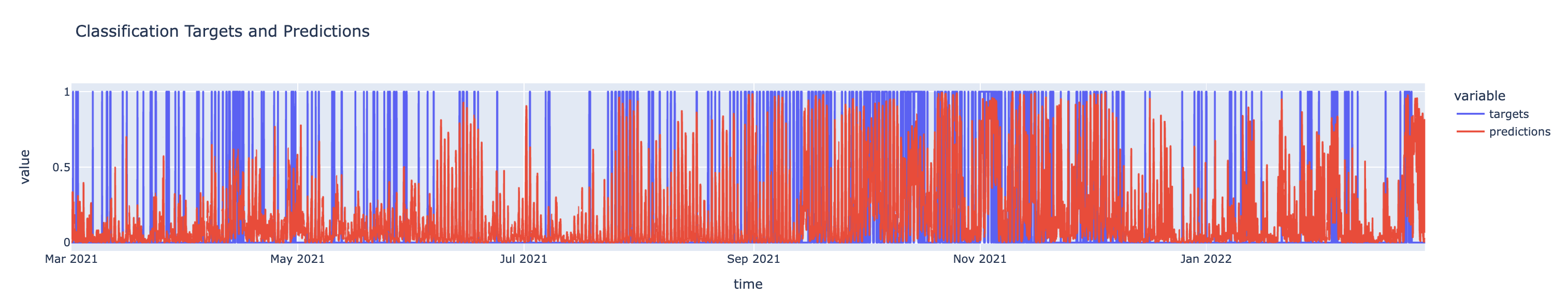
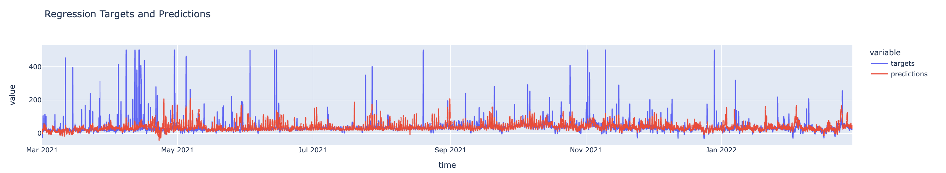
Take note that the targets in the plot below cap out at $500 because of the clipping we did above. When we properly evaluate this model, we'll need to pull in the raw (un-clipped) System Lambda time series.
px.line(regression_result, y=["targets", "predictions"], title="Regression Targets and Predictions")
The backtest results give us some metrics for our models, but it would be nice to contextualize those against some simple baselines. The two baseline's we'll conider are:
- Same as today's DAM price
- Same as yesterday's RTM price
We can pull these baselines from our graph, once we deploy it and run the corresponding nodes. We'll pull the raw System Lambda time series here too. Running these time series will trigger the data to be queried for our requested time range. It'll get written to Myst's time series database and be available for querying here.
The code below waits on the data query jobs to be completed, so it may take a moment. You can monitor the status of the created jobs in the Myst Platform UI.
def create_baseline_pandas_series(time_series: myst.TimeSeries) -> pandas.Series:
    """Creates a pandas series with the historical data for the baseline."""
    run_job = time_series.run(
        start_timing=myst.Time("2021-03-01T06:00:00Z"), end_timing=myst.Time("2022-03-01T06:00:00Z")
    )
    run_job = run_job.wait_until_completed()

    run_result = time_series.get_run_result(uuid=run_job.result)
    pandas_series = run_result.outputs[0].flatten().to_pandas_series()

    return pandas_series


# Ensure that our project is deployed so we can generate ad hoc runs.
project.deploy(title="System Lambda Price Spike Deployment")

# Create the pandas series containing the historical data for the baselines.
system_lambda = create_baseline_pandas_series(
    time_series=get_time_series_by_title(nodes=project.list_nodes(), title="System Lambda")
)

system_lambda_persistence = create_baseline_pandas_series(
    time_series=get_time_series_by_title(nodes=project.list_nodes(), title="System Lambda - Lag PT48H")
)
system_lambda_persistence.rename("System Lambda - 48H Persistence")

system_lambda_da_persistence = create_baseline_pandas_series(
    time_series=get_time_series_by_title(nodes=project.list_nodes(), title="System Lambda DA - Lag PT24H")
)
system_lambda_da_persistence.rename("System Lambda DA - 24H Persistence")
Now that we have baselines, Myst platform predictions, and targets, we can compare metrics. We'll look at precision, recall, and AUC across the baselines and the two models for the task of predicting when price will spike above $50.
We'll also take a look a MSE and MAE for the two baselines and the regression model to contextualize its performance on predicting the price directly.
classification_metrics = []
regression_metrics = []

# Extract the classification and regression targets and predictions.
classification_targets = classification_result["targets"]
classification_predictions = classification_result["predictions"].rename("Myst Price Spike Probability")
regression_targets = system_lambda
regression_predictions = regression_result["predictions"].rename("Myst Price Forecasts")

# Compute the regression and classification metrics.
for predictions in (
    system_lambda_da_persistence,
    system_lambda_persistence,
    classification_predictions,
    regression_predictions,
):
    if "Probability" not in predictions.name:
        mse = sklearn.metrics.mean_squared_error(y_true=regression_targets, y_pred=predictions)
        mae = sklearn.metrics.mean_absolute_error(y_true=regression_targets, y_pred=predictions)
        regression_metrics.append(pandas.Series(index=["MSE", "MAE"], data=[mse, mae], name=predictions.name))

    # For price-valued time series, we'll predict "spiking" when the price > 50,
    # the same way price spikes are defined for the classification model.
    threshold = 50

    # For probability-valued time series, we'll use a 0.5 threshold.
    # This could be tuned on a validation set to achieve a desired precision-recall tradeoff.
    if "Probability" in predictions.name:
        threshold = 0.50

    precision = sklearn.metrics.precision_score(y_true=classification_targets, y_pred=predictions > threshold)
    recall = sklearn.metrics.recall_score(y_true=classification_targets, y_pred=predictions > threshold)
    auc = sklearn.metrics.roc_auc_score(y_true=classification_targets, y_score=predictions)

    classification_metrics.append(
        pandas.Series(index=["Precision", "Recall", "AUC"], data=[precision, recall, auc], name=predictions.name)
    )

regression_metrics_df = pandas.concat(regression_metrics, axis=1).T
classification_metrics_df = pandas.concat(classification_metrics, axis=1).T
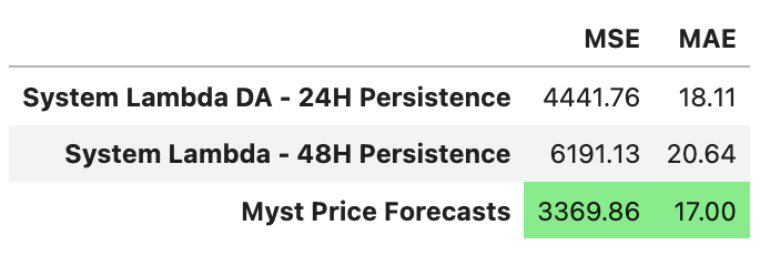
Finally, we can now view the metrics of our models against the baselines we defined.
regression_metrics_df.style.format(precision=2).highlight_min(color="lightgreen", axis=0)
classification_metrics_df.style.format(precision=2).highlight_max(color="lightgreen", axis=0)
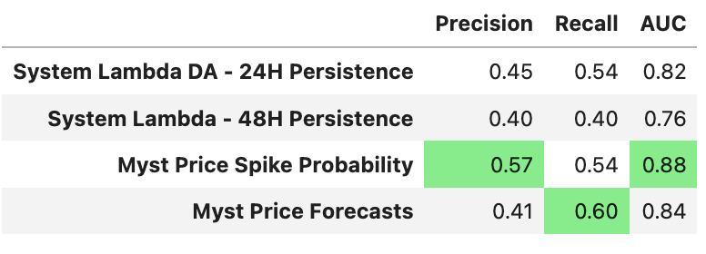
We find that both Myst forecasts beat our simple baselines, and that the probability forecast yields the best AUC metric on the System Lambda > $50 task.
Deploy your NoTS
Since we can now feel confident in our model's performance, you can go ahead and deploy this project. Before doing so, you have to add model fit and time series run policies. These policies determine how often your models should be retrained, and how frequently new forecasts should be generated.
def create_fit_policy(model: myst.Model) -> None:
    """Creates a fit policy to the specified model."""
    model.create_fit_policy(
        schedule_timing=myst.CronTiming(cron_expression="0 0 * * *", time_zone=TIME_ZONE),
        start_timing=myst.Time("2017-01-01T06:00:00Z"),
        end_timing=myst.TimeDelta("-P1D"),
    )


def create_predict_policy(forecast: myst.TimeSeries) -> None:
    """Creates a run policy to the specified forecast time series."""
    forecast.create_run_policy(
        schedule_timing=myst.CronTiming(cron_expression="0 9 * * *", time_zone=TIME_ZONE),
        start_timing=myst.TimeDelta("PT15H"),
        end_timing=myst.TimeDelta("PT39H"),
    )


# We need to add fit and predict policies to our models and forecasts in order to deploy the project and run nodes.
# Deploying a project indicates to Myst that we should start storing data associated with the project. You can always
# deactivate and/or delete your project if you don't want it to make recurring forecasts.
create_fit_policy(classification_model)
create_fit_policy(regression_model)
create_predict_policy(spike_probability_forecast)
create_predict_policy(price_forecast)

project.deploy(title="System Lambda Price Spike Deployment")
Updated over 3 years ago